Event studies
We look at Sun and Abraham.
- they raise concerns with dynamic specification typicaly used
- estimated parameters might not be the average of positively weighted well defined causal effects
- can contaminate pre-trends as well as main estimates
We consider an event study framework.
CATT_{e, \ell} = E[Y_{i, e + \ell} - Y_{i, e + \ell}(\infty)|E_i = e]
- for $l \geq 0 $ these are ATT:
l\geq 0 , \quad CATT_{e, \ell} = E[Y_{i, e + \ell}(e) - Y_{i, e + \ell}(\infty)|E_i = e]
- for $l < 0 $, under the no anticipation assumption, they end up being 0
l<0, \quad CATT_{e, \ell} = E[Y_{i, e + \ell}(\infty) - Y_{i, e + \ell}(\infty)|E_i = e] = 0
Y_{i, t} = \alpha_i + \lambda_t + \sum_{\ell \in \mathcal{G}} \mu_{\ell} D^{\ell}_{i, t} + \nu_{i, t} \tag{1}
-
The \mu_{\ell} can be decomposed as
$$
\mu_{\ell} = \sum_{e, \ell'}\omega_{e, \ell'}^{\ell} CATT_{e, \ell'} \tag{2}
$$
-
In general, the \omega's from (2) can be estimated through the regressions that are ran separatly of each value of e and l:
$$
D_{i, t}^{\ell} \cdot \mathbb{1} {E_i = e} = \alpha_i + \lambda_t + \sum_{g \in \mathcal{G}} \omega_{e, \ell}^g \mathbb{1}{t - E_i \in g} + u_{i, t} \tag{4}
$$
A simple example from the paper
We consider a simple case with T = 0,1,2 and cohorts E_i \in \{1, 2, \infty\}.
We define g^{incl} = \{−2, 0\} and g^{excl} = \{−1, 1\}
- exclude -1 to normalize relative to -1
- exclude 1 to drop "distant" lags.
In the simple case we consider, if all individuals are treated we have
$$
\mu_{-2} = \underbrace{CATT_{2, -2}}{\text{own period}} + \underbrace{\frac{1}{2}CATT - \frac{1}{2}CATT_{2, 0}}{\ell' \in g^{incl}, \ell' \neq -2} + \underbrace{\frac{1}{2}CATT - CATT_{1, -1} - \frac{1}{2}CATT_{2, -1}}_{\ell' \in g^{excl}} \tag{5}
$$
- With no anticipation we get that $CATT_{e,l} = 0 $ for l<0 and so we get:
\mu_{-2} = \underbrace{\frac{1}{2}CATT_{1, 0} - \frac{1}{2}CATT_{2, 0}}_{\ell' \in g^{incl}, \ell' \neq -2} + \underbrace{\frac{1}{2}CATT_{1, 1}}_{\ell' \in g^{excl}} \tag{5}
- We can still get non zero \mu_{-2} even in the absence of anticipation effects!
- This is true even in the case where CATT are homogenous.
Generating panel data
| import numpy as np
import pandas as pd
import statsmodels.formula.api as smf
from matplotlib import pyplot as plt
import tqdm
|
1
2
3
4
5
6
7
8
9
10
11
12
13
14
15
16
17
18
19
20
21
22
23
24
25
26
27
28
29
30
31
32
33
34
35
36
37
38
39
40
41
42
43
44
45
46
47
48
49
50
51
52
53
54
55
56
57
58 | def gen_panel(share_treated, CATT):
'''
Purpose:
Generate panel data.
Inputs:
share_treated (float): integer multiple of 0.01 in (0, 1]
CATT (dict): dictionary giving CATT values
Returns:
panel (Pandas DataFrame)
'''
T = 2
N = 200
n_treated = N * share_treated
CATT_E1_lm1 = CATT['CATT_E1_lm1']
CATT_E1_l0 = CATT['CATT_E1_l0']
CATT_E1_lp1 = CATT['CATT_E1_lp1']
CATT_E2_lm2 = CATT['CATT_E2_lm2']
CATT_E2_lm1 = CATT['CATT_E2_lm1']
CATT_E2_l0 = CATT['CATT_E2_l0']
panel = pd.DataFrame()
panel['t'] = np.tile(np.array(np.arange(T + 1)), N)
panel['i'] = np.repeat(np.arange(N), T + 1)
# Add individual and time effects
panel['alpha_i'] = np.repeat(np.random.random(size=(N)), T + 1)
panel['lambda_t'] = np.tile(np.random.random(size=(T + 1)), N)
# Set half the treated to E_1 and the other half to E_2
panel.eval(
'E = (i < ({} // 2)) + 2 * (({} // 2) <= i < {})'.format(n_treated,n_treated,n_treated)
, inplace=True)
panel.loc[panel['E'] == 0, 'E'] = 100 # Set very large
# Generate Y
panel.eval(
'Y = (E == 1) * ('
'@CATT_E1_lm1 * (t == 0)'
'+ @CATT_E1_l0 * (t == 1)'
'+ @CATT_E1_lp1 * (t == 2)'
') +'
'(E == 2) * ('
'@CATT_E2_lm2 * (t == 0)'
'+ @CATT_E2_lm1 * (t == 1)'
'+ @CATT_E2_l0 * (t == 2)'
') + alpha_i + lambda_t'
, inplace=True)
# Add group-specific means to alpha_i
panel.loc[panel['E'] == 1, 'Y'] += 0.3 #np.random.random()
panel.loc[panel['E'] == 2, 'Y'] += 0.2 #np.random.random()
panel.loc[panel['E'] == 100, 'Y'] += 0 #np.random.random()
# Generate D
panel.eval('D_lm2 = 1 * (t - E == -2)', inplace=True)
panel.eval('D_l0 = 1 * (t - E == 0)', inplace=True)
return panel
|
Viewing some panel data
 1
 2
 3
 4
 5
 6
 7
 8
 9
10
11
12
13
14
15
16
17
18
19
20
21
22 | # Choose share_treated
share_treated = 0.03
# Generate CATT
CATT_E1_lm1 = 0 # no anticipation
CATT_E1_l0 = 0.4 # np.random.random()
CATT_E1_lp1 = 0.8 #np.random.random()
CATT_E2_lm2 = 0 # no anticipation
CATT_E2_lm1 = 0 # no anticipation
CATT_E2_l0 = 0.6 #np.random.random()
CATT = {
'CATT_E1_lm1': CATT_E1_lm1,
'CATT_E1_l0': CATT_E1_l0,
'CATT_E1_lp1': CATT_E1_lp1,
'CATT_E2_lm2': CATT_E2_lm2,
'CATT_E2_lm1': CATT_E2_lm1,
'CATT_E2_l0': CATT_E2_l0}
# Generate panel
panel = gen_panel(share_treated, CATT)
display(panel.head(n=20))
|
|
t |
i |
alpha_i |
lambda_t |
E |
Y |
D_lm2 |
D_l0 |
| 0 |
0 |
0 |
0.982422 |
0.909437 |
1.0 |
2.191859 |
0.0 |
0.0 |
| 1 |
1 |
0 |
0.982422 |
0.144418 |
1.0 |
1.826840 |
0.0 |
1.0 |
| 2 |
2 |
0 |
0.982422 |
0.470141 |
1.0 |
2.552563 |
0.0 |
0.0 |
| 3 |
0 |
1 |
0.605144 |
0.909437 |
1.0 |
1.814581 |
0.0 |
0.0 |
| 4 |
1 |
1 |
0.605144 |
0.144418 |
1.0 |
1.449562 |
0.0 |
1.0 |
| 5 |
2 |
1 |
0.605144 |
0.470141 |
1.0 |
2.175285 |
0.0 |
0.0 |
| 6 |
0 |
2 |
0.774368 |
0.909437 |
1.0 |
1.983805 |
0.0 |
0.0 |
| 7 |
1 |
2 |
0.774368 |
0.144418 |
1.0 |
1.618786 |
0.0 |
1.0 |
| 8 |
2 |
2 |
0.774368 |
0.470141 |
1.0 |
2.344509 |
0.0 |
0.0 |
| 9 |
0 |
3 |
0.534308 |
0.909437 |
2.0 |
1.643745 |
1.0 |
0.0 |
| 10 |
1 |
3 |
0.534308 |
0.144418 |
2.0 |
0.878726 |
0.0 |
0.0 |
| 11 |
2 |
3 |
0.534308 |
0.470141 |
2.0 |
1.804449 |
0.0 |
1.0 |
| 12 |
0 |
4 |
0.784083 |
0.909437 |
2.0 |
1.893520 |
1.0 |
0.0 |
| 13 |
1 |
4 |
0.784083 |
0.144418 |
2.0 |
1.128501 |
0.0 |
0.0 |
| 14 |
2 |
4 |
0.784083 |
0.470141 |
2.0 |
2.054224 |
0.0 |
1.0 |
| 15 |
0 |
5 |
0.178669 |
0.909437 |
2.0 |
1.288106 |
1.0 |
0.0 |
| 16 |
1 |
5 |
0.178669 |
0.144418 |
2.0 |
0.523086 |
0.0 |
0.0 |
| 17 |
2 |
5 |
0.178669 |
0.470141 |
2.0 |
1.448810 |
0.0 |
1.0 |
| 18 |
0 |
6 |
0.727277 |
0.909437 |
100.0 |
1.636714 |
0.0 |
0.0 |
| 19 |
1 |
6 |
0.727277 |
0.144418 |
100.0 |
0.871695 |
0.0 |
0.0 |
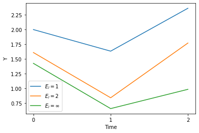
Plotting Y over time, grouped by E
| panel_sum = panel.groupby(['E', 't'])['Y'].mean()
plt.plot(range(3), panel_sum[:3], label='$E_i=1$')
plt.plot(range(3), panel_sum[3:6], label='$E_i=2$')
plt.plot(range(3), panel_sum[6:9], label='$E_i = \infty$')
plt.xlabel('Time')
plt.xticks([0,1,2])
plt.ylabel('Y')
plt.legend()
plt.show()
|
Computing the weights
Recall that the \omega's from (2) can be estimated through the regressions for each (e,\ell)
$$
D_{i, t}^{\ell} \cdot \mathbb{1} {E_i = e} = \alpha_i + \lambda_t + \sum_{g \in \mathcal{G}} \omega_{e, \ell}^g \mathbb{1}{t - E_i \in g} + \nu_{i, t} \tag{4}
$$
1
2
3
4
5
6
7
8
9
10
11
12
13
14
15
16
17
18
19
20
21
22
23
24
25
26
27
28
29
30
31
32
33 | def get_weights(panel):
'''
Purpose:
Compute the weights using OLS.
Inputs:
panel (Pandas DataFrame): panel to compute weights
Returns:
gm2 (dict)
g0 (dict)
'''
gm2 = {}
g0 = {}
# We loop over e and l
for e in [1, 2]:
for l in range(-2, 2):
# Avoid out-of-bounds cases
if not (((e == 1) and (l == -2)) or ((e == 2) and (l == 1))):
# construct the regressors as in equation (4)
panel.eval('D = 1 * ((t - E == @l) & (E == @e))', inplace=True)
panel.eval('gm2 = (t - E) == -2', inplace=True)
panel.eval('g0 = (t - E) == 0', inplace=True)
# run the regression as in equation (4)
ols = smf.ols('D ~ C(t) + C(i) + gm2 + g0', panel)
ols_result = ols.fit().params
# collect the parameters
gm2[(e, l)] = ols_result['gm2[T.True]']
g0[(e, l)] = ols_result['g0[T.True]']
return gm2, g0
|
Apply the functions
 1
 2
 3
 4
 5
 6
 7
 8
 9
10
11
12
13
14
15
16
17
18
19
20
21
22
23
24
25
26
27
28
29
30
31
32
33
34
35
36
37
38
39
40
41
42
43
44
45
46
47 | # Loop over share_treated
share_treated = np.linspace(0.01, 1, 20)
mu_lm2 = []
CATT_mu_lm2 = []
gm2_full = {}
g0_full = {}
for share in tqdm.tqdm(share_treated):
panel = gen_panel(share, CATT)
# Use Y from panel to estimate mu_l
# -1 to drop constant
ols = smf.ols('Y ~ C(i) + C(t) + D_lm2 + D_l0 -1', panel)
ols_result = ols.fit().params
# Extract each of the weights for all (e,l) combinations
gm2, g0 = get_weights(panel)
wt_E2_lm2 = gm2[(2, -2)]
wt_E1_l0 = gm2[(1, 0)]
wt_E2_l0 = gm2[(2, 0)]
wt_E1_lp1 = gm2[(1, 1)]
wt_E1_lm1 = gm2[(1, -1)]
wt_E2_lm1 = gm2[(2, -1)]
# Save results
mu_lm2.append(ols_result['D_lm2'])
CATT_mu_lm2.append(wt_E2_lm2 * CATT_E2_lm2
+ wt_E1_l0 * CATT_E1_l0
+ wt_E2_l0 * CATT_E2_l0
+ wt_E1_lp1 * CATT_E1_lp1
+ wt_E1_lm1 * CATT_E1_lm1
+ wt_E2_lm1 * CATT_E2_lm1)
# Append weights to gm2, g0
for key in gm2.keys():
try:
gm2_full[key].append(gm2[key])
except:
gm2_full[key] = [gm2[key]]
for key in g0.keys():
try:
g0_full[key].append(g0[key])
except:
g0_full[key] = [g0[key]]
|
| 100%|██████████| 20/20 [00:05<00:00, 3.93it/s]
|
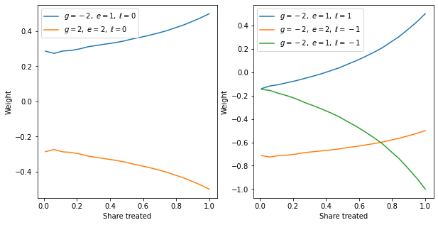
Graph the weights for different treated shares
 1
 2
 3
 4
 5
 6
 7
 8
 9
10
11
12
13
14
15
16
17 | plt.figure(figsize=(10,5))
plt.subplot(1,2,1)
plt.plot(share_treated, gm2_full[(1, 0)], label='$g=-2,\; e=1,\; \ell=0$')
plt.plot(share_treated, gm2_full[(2, 0)], label='$g{=}2,\; e{=}2,\; \ell{=}0$')
plt.xlabel('Share treated')
plt.ylabel('Weight')
plt.legend()
plt.subplot(1,2,2)
plt.plot(share_treated, gm2_full[(1, 1)], label='$g=-2,\; e=1,\; \ell=1$')
plt.plot(share_treated, gm2_full[(2, -1)], label='$g=-2,\; e=2,\; \ell=-1$')
plt.plot(share_treated, gm2_full[(1, -1)], label='$g=-2,\; e=1,\; \ell=-1$')
plt.xlabel('Share treated')
plt.ylabel('Weight')
plt.legend()
plt.show()
|
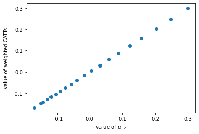
Using true CATT to check weights
| plt.plot(np.array(mu_lm2), np.array(CATT_mu_lm2),'o', label='OLS mu versus weighted mu')
plt.xlabel('value of $\mu_{-2}$')
plt.ylabel('value of weighted CATTs')
plt.show()
|
Estimating the CATTs
We estimate the CATTs using the following regression:
$$
Y_{i, t} = \alpha_i + \lambda_t + \sum_{e \notin C} \sum_{\ell \neq -1} \delta_{e, \ell}(\mathbb{1}{E_i = e} \cdot D_{i, t}^{\ell}) + \epsilon_{i, t} \tag{6}
$$
where in this case, C = \{\infty\} gives that the never-treated group serves as the cohort we exclude (if there are no never-treated groups, C could include the last treated group, and any always-treated cohorts must be included in C) and we treat \ell = -1 as a baseline.
\hat{\delta}_{e, \ell} gives a DID estimator for CATT_{e, \ell}.
1
2
3
4
5
6
7
8
9
10
11
12
13
14
15
16 | # Set share_treated in (0, 1)
share_treated = 0.1
panel = gen_panel(share_treated, CATT)
panel.eval('delta_E1_l0 = 1 * ((t - E == 0) & (E == 1))', inplace=True)
panel.eval('delta_E1_lp1 = 1 * ((t - E == 1) & (E == 1))', inplace=True)
panel.eval('delta_E2_lm2 = 1 * ((t - E == -2) & (E == 2))', inplace=True)
panel.eval('delta_E2_l0 = 1 * ((t - E == 0) & (E == 2))', inplace=True)
ols = smf.ols('Y ~ C(i) + C(t) + delta_E1_l0 + delta_E1_lp1 + delta_E2_lm2 + delta_E2_l0 -1', panel)
ols_result = ols.fit().params
delta_E1_l0 = ols_result['delta_E1_l0']
delta_E1_lp1 = ols_result['delta_E1_lp1']
delta_E2_lm2 = ols_result['delta_E2_lm2']
delta_E2_l0 = ols_result['delta_E2_l0']
|
 1
 2
 3
 4
 5
 6
 7
 8
 9
10
11
12
13
14
15
16
17 | # Compare to truth:
print('CATT_E1_l0:', CATT_E1_l0)
print('CATT_E1_lp1:', CATT_E1_lp1)
print('CATT_E2_lm2:', CATT_E2_lm2)
print('CATT_E2_l0:', CATT_E2_l0)
# Estimates:
print('delta_E1_l0:', delta_E1_l0)
print('delta_E1_lp1:', delta_E1_lp1)
print('delta_E2_lm2:', delta_E2_lm2)
print('delta_E2_l0:', delta_E2_l0)
# # Differences:
# print('E1_l0:', delta_E1_l0 - CATT_E1_l0)
# print('E1_lp1:', delta_E1_lp1 - CATT_E1_lp1)
# print('E2_lm2:', delta_E2_lm2 - CATT_E2_lm2)
# print('E2_l0:', delta_E2_l0 - CATT_E2_l0)
|
| CATT_E1_l0: 0.4
CATT_E1_lp1: 0.8
CATT_E2_lm2: 0
CATT_E2_l0: 0.6
delta_E1_l0: 0.4000000000000064
delta_E1_lp1: 0.8000000000000045
delta_E2_lm2: 9.764199571088277e-15
delta_E2_l0: 0.6000000000000056
|
- how to construct inference on average over cohort (inference on linear combination of parameters)
- how to include covariates