In this problem set we are going to make use of pandas to analyze the effect of a fictuous experiment I have added to a data set. The data will be using is the sample data provided by Yelp. The goal is to familiarize ourselves with working with such datasets.

The original data is available here: Yelp data. However for this homework you will have to use the data I constructed from the original sample. You can download such file here:

homework data: hw-yelp.tar.gz (~2.6Go)

Note that on windows you can use 7zip to uncompress that file. On OSX and linux you can simply use tar -cxvf hw-yelp.tar.gz

In the data I have introduced an experiment. The back sotry is that Yelp rolled out a new interface for a randomly select group of users. These uses were randomly selected among users that posted a review in the month of January 2010. The id of these users in listed in the yelp_academic_dataset_review_treatment.json file present in the archive.

For this group of user a the new website interface was put in place on February 1st 2010. As a Yelp employee you are asked to analyze the impact of a new app. The company is interested in the effect on user engagement which is measured by rating activity. We will focus on the number of ratings.

In this homework we will cover: 1. loading large data using streaming/chunks, learn about json - working with date in pandas - analyze randomly assigned treatment - construct comparable control group - analyze at the level of randomization

some useufl links: - tutorial on dates in pandas - pandas documentation on reshaping - yelp data documentation

We start with a simple list of imports, as well as defining the path to the file we will be using. Please update the paths to point to the correct location on your computer.

import os
import pandas as pd
import tqdm
import seaborn as sns
import matplotlib.pyplot as plt
import numpy as np

file_review = os.path.expanduser("~/Downloads/hw-yelp/yelp_academic_dataset_review_experiment.json")
file_treatment = os.path.expanduser("~/Downloads/hw-yelp/yelp_academic_dataset_review_treatment.json")

def file_len(fname):
    """ Function which efficiently computes the number of lines in file"""
    with open(fname) as f:
        for i, l in enumerate(f):
            pass
    return i + 1

You are already familiar with the following section, this is the code that loads my solution. Since you don't have the file, this part of the code won't work for you.

%cd ..
%load_ext autoreload
%autoreload 2
import solutions.sol_pset3 as solution # you need to command this, you don't have the solution file!

/Users/thibautlamadon/git/econ-21340

Loading the yelp review data

The data is stored in json format. This is a widely used format to store structured data. See here for working with json in general in python.

The data itself is quite large, hence we are going to use the chunksize argument of the read_json function of pandas. You can of course try for your self to directly load the data by using pd.read_json(file_review), this however might take a while!

In the following section I provide a code example that loads the business information using chunks of size 100,000. The code contains a few errors. Use the data documentation (using the link in the intro) to fix the code a load the data. The code also drops variables which will be very needed and keep some others that are just going to clutter your computer memory. Again, look at the documentation and at the questions ahead to keep the right set of variables.

Note how the code first compute the length of the file

size = 100000
review = pd.read_json(filepath, lines=True,
                      dtype={'review_id':str,
                             'user_id':float,
                             'business_id':str,
                             'stars':int,
                             'date':str,
                             'text':float,
                             'useful':int,
                             'funny':str,
                             'cool':int},
                      chunksize=size)

chunk_list = []
for chunk_review in tqdm.tqdm(review,total=  np.ceil(file_len(filepath)/size )  ):
    # Drop columns that aren't needed
    chunk_review = chunk_review.drop(['review_id','date'], axis=1)
    chunk_list.append(chunk_review)

df = pd.concat(chunk_list, ignore_index=True, join='outer', axis=0)

The following runs my version of the code, it takes around 2 minutes on my laptop. I show you a few of the columns that I chose to extract. In particular, you can check that you get the right row count of 7998013.

df_review = solution.question1(file_review)
df_review['date'] = pd.to_datetime(df_review.date) # convert the date string to an actual date
df_review[['review_id','user_id','date']]

100%|██████████| 80/80.0 [02:16<00:00,  1.71s/it]

	review_id	user_id	date
0	xQY8N_XvtGbearJ5X4QryQ	OwjRMXRC0KyPrIlcjaXeFQ	2015-04-15 05:21:16
1	UmFMZ8PyXZTY2QcwzsfQYA	nIJD_7ZXHq-FX8byPMOkMQ	2013-12-07 03:16:52
2	LG2ZaYiOgpr2DK_90pYjNw	V34qejxNsCbcgD8C0HVk-Q	2015-12-05 03:18:11
3	i6g_oA9Yf9Y31qt0wibXpw	ofKDkJKXSKZXu5xJNGiiBQ	2011-05-27 05:30:52
4	6TdNDKywdbjoTkizeMce8A	UgMW8bLE0QMJDCkQ1Ax5Mg	2017-01-14 21:56:57
...	...	...	...
7998008	LAzw2u1ucY722ryLEXHdgg	6DMFD3BRp-MVzDQelRx5UQ	2019-12-11 01:07:06
7998009	gMDU14Fa_DVIcPvsKtubJA	_g6P8H3-qfbz1FxbffS68g	2019-12-10 04:15:00
7998010	EcY_p50zPIQ2R6rf6-5CjA	Scmyz7MK4TbXXYcaLZxIxQ	2019-06-06 15:01:53
7998011	-z_MM0pAf9RtZbyPlphTlA	lBuAACBEThaQHQGMzAlKpg	2018-07-05 18:45:21
7998012	nK0JGgr8aO4mcFPU4pDOEA	fiA6ztHPONUkmX6yKIXyHg	2019-12-07 00:29:55

7998013 rows × 3 columns

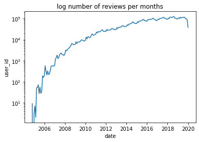
Our first plot of the data

Next, to get a sense of the data, we plot the user engagement over time. For this I ask you to plot the log number of reviews per month using our created data.

To get to the result I recommend you look into either the resample menthod or the grouper method. If you are not too familiar with them, I added a link at the top to a great tutorial.

solution.question2(df_review)

png

A randomized experiment

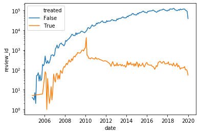
We now want to extract our experimental data from our large data set. Given the random assignment we are going to compare the treated group to simply everyone else in the data. In this exercice, we are interested in the effect of the policy overt time. We are then going to look at the log number of reviews in each of the month around the introduction of the interface change.

I would like for you to do the following: 1. extract the list of treated individuals from the provided file 2. attach the treated status to each observation in the data, you can use eval or a merge. 3. plot the log number of reviews per month in the treatment and in the control group. 4. given that the treatment status was randomized, the picture should look a bit surpising, please explain what you would have expected to see.

Here is the plot I get, try to reproduce it as closely as possible.

# df_local returns all entries with a column treated, user_treat is the list of treated user_id
user_treat,df_local = solution.question3(df_review, file_treatment)

png

df_local

	review_id	user_id	business_id	stars	date	treated	control
0	xQY8N_XvtGbearJ5X4QryQ	OwjRMXRC0KyPrIlcjaXeFQ	-MhfebM0QIsKt87iDN-FNw	2	2015-04-15 05:21:16	False	False
1	UmFMZ8PyXZTY2QcwzsfQYA	nIJD_7ZXHq-FX8byPMOkMQ	lbrU8StCq3yDfr-QMnGrmQ	1	2013-12-07 03:16:52	False	False
2	LG2ZaYiOgpr2DK_90pYjNw	V34qejxNsCbcgD8C0HVk-Q	HQl28KMwrEKHqhFrrDqVNQ	5	2015-12-05 03:18:11	False	False
3	i6g_oA9Yf9Y31qt0wibXpw	ofKDkJKXSKZXu5xJNGiiBQ	5JxlZaqCnk1MnbgRirs40Q	1	2011-05-27 05:30:52	False	False
4	6TdNDKywdbjoTkizeMce8A	UgMW8bLE0QMJDCkQ1Ax5Mg	IS4cv902ykd8wj1TR0N3-A	4	2017-01-14 21:56:57	False	False
...	...	...	...	...	...	...	...
7998008	LAzw2u1ucY722ryLEXHdgg	6DMFD3BRp-MVzDQelRx5UQ	XW2kaXdahICaJ27A0dhGHg	1	2019-12-11 01:07:06	False	False
7998009	gMDU14Fa_DVIcPvsKtubJA	_g6P8H3-qfbz1FxbffS68g	IsoLzudHC50oJLiEWpwV-w	3	2019-12-10 04:15:00	False	False
7998010	EcY_p50zPIQ2R6rf6-5CjA	Scmyz7MK4TbXXYcaLZxIxQ	kDCyqlYcstqnoqnfBRS5Og	5	2019-06-06 15:01:53	False	False
7998011	-z_MM0pAf9RtZbyPlphTlA	lBuAACBEThaQHQGMzAlKpg	VKVDDHKtsdrnigeIf9S8RA	3	2018-07-05 18:45:21	False	False
7998012	nK0JGgr8aO4mcFPU4pDOEA	fiA6ztHPONUkmX6yKIXyHg	2SbyRgHWuWNlq18eHAx95Q	5	2019-12-07 00:29:55	False	False

7998013 rows × 7 columns

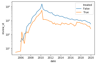
Changing comparaison group

We clearly created some issues in the way we analyzed our sample. In this section we are going to use a more comparable group.

using the criteria descriged in the intro, construct the original set of users from which the treatment group was selected.
extracts the users from the this group wich are not in the treatment group, this will be our control group.
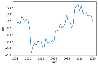
using this new control group, plot the log number of reviews in each quarter for treatment and control
finally plot the outcome in difference, however make sure to remove the log-number of individual from each group to plot the log number of reviews per user, overwise your intercept won't be around 0!

Here are the plots I got:

df_local = solution.question4(df_local,user_treat)

png

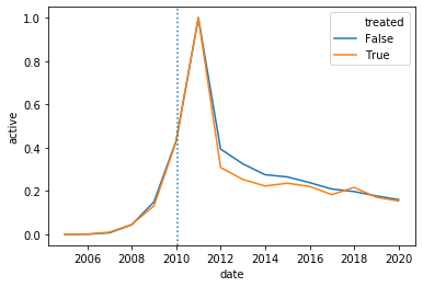
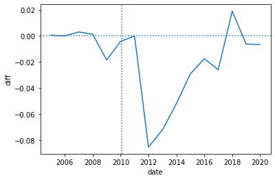
Using activity per user and time

We are now interested in conducting some inference on our results. However we remember that the level of randomization is the user not the review. Hence we now decide to construct observation at the (user,year) level. We decide to use years instead of months because the probability at the month level is too low.

Construct a DataFrame with all (user,year) pairs and a column called post which is equal to 1 if the user posted in that month and 0 if he didn't. To construct such dataframe I used the pd.MultiIndex.from_product function, but one could use a merge instead.
Use this newly created DataFrame to plot the level for each group and each, and to plot the difference between the two.

Here are the plots I constructed:

df_local_user = solution.question5(df_local,user_treat)

png

df_local_user

	user_id	date	treated	review_id	post
0	--J8UruLD_xvVuI1lMAxpA	2010-12-31	False	1	True
1	--J8UruLD_xvVuI1lMAxpA	2012-12-31	False	1	True
2	--J8UruLD_xvVuI1lMAxpA	2009-12-31	False	0	False
3	--J8UruLD_xvVuI1lMAxpA	2011-12-31	False	0	False
4	--J8UruLD_xvVuI1lMAxpA	2014-12-31	False	0	False
...	...	...	...	...	...
77531	zznOF_-TAaCRw1lRVQ9GzQ	2007-12-31	False	0	False
77532	zznOF_-TAaCRw1lRVQ9GzQ	2008-12-31	False	0	False
77533	zznOF_-TAaCRw1lRVQ9GzQ	2006-12-31	False	0	False
77534	zznOF_-TAaCRw1lRVQ9GzQ	2005-12-31	False	0	False
77535	zznOF_-TAaCRw1lRVQ9GzQ	2004-12-31	False	0	False

77536 rows × 5 columns

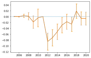
Construct confidence inference

In this final question our goal is to add some inference to our plot. We are going to simply use the asymptotic variance implied by the OLS formula. Do the following:

create a function that will take a dataframe containing the columns post and treat and returns the OLS estimate of post on treat together with the estimate of the variance of that estimate (Remember that in this simple case $\hat{\beta} = cov(y,x)/var(x)$ and that teh variance is $\sigma^2_\epsilon/(n \cdot var(x))$ . Return the results as a new dataframe with one row and 2 columns.
apply your function to your data from question 4 within eave year (you can do that using pd.Grouper(freq='Y',key='date') within a groupby and use the apply method.
use your grouped results to plot the mean together with their 95% asymptotic conf interval
comment on the results, in particular on date before the start of the experiment.

I report the plot I got:

import matplotlib
matplotlib.rcParams.update({'errorbar.capsize': 3})
solution.question6(df_local_user)

png

Congrats, you are done!