A homework on mulitway fixed effect approach
In this homework we are going to consider a fictuous grading at a given universities and try to see what we can learn from grade variability and it affects earnings.
In the first data set we have the grades collected by a bunch of student within a given summester. Each student attended 2 courses. From this data we are going to try to extrac the ability of each student while allowing for course specific intercept. We can then use this to evaluate how much of the grade variation is due to student differences versus course differences and other factors (residuals).
Given this ability measures, we then merge a second file which has the earnings of the student at age 35. We then evaluate the effect of academic ability on individual earnings. Here again we will worry about the effect of over-fitting.
Of course this requires, like we saw in class, estimating many parameters, hence we will look into overfitting and how to address it! We wil lmake use of sparse matrices, degree of freedom correction and bias correction.
The two data files you will need are:
- grades: hw4-grades.json
- earnings: hw4-earnings.json
Useful links: - Sparse linear solver
import os
import pandas as pd
import tqdm
import seaborn as sns
import matplotlib.pyplot as plt
import numpy as np
%cd ..
%load_ext autoreload
%autoreload 2
/home/tlamadon/git/econ-21340
import solutions.sol_pset4 as solution # you need to command this, you don't have the solution file!
#solution.simulate_data()
Explaining the dispersion in grades
Load the grade data from hw4-grades.json. Then compute:
- total variance in grades
- the between class variance
- plot the histogram of class size
df_all = solution.question1()

ns = len(np.unique(df_all['student_id']))
nc = len(np.unique(df_all['class_id']))
nn = len(df_all)

print("{} students and {} classes".format(ns,nc))

df_all[["grade","class_id","student_id","major","firstname"]]
 total variance is 2.1867408049173007
 between class variance is 0.7541357576225806
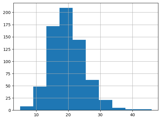
6732 students and 673 classes
| grade | class_id | student_id | major | firstname | |
|---|---|---|---|---|---|
| 0 | -3.099938 | MQ2281 | 5 | SOCIAL SCIENCE OR HISTORY TEACHER EDUCATION | Francis |
| 1 | -3.021075 | JP1499 | 5 | SOCIAL SCIENCE OR HISTORY TEACHER EDUCATION | Francis |
| 2 | -0.042223 | HO0525 | 20 | ELEMENTARY EDUCATION | Cruz |
| 3 | -1.842850 | BZ6573 | 20 | ELEMENTARY EDUCATION | Cruz |
| 4 | 0.038426 | FM1995 | 21 | MISCELLANEOUS PSYCHOLOGY | Denise |
| ... | ... | ... | ... | ... | ... |
| 13459 | -2.082608 | JH2331 | 50684 | COMMUNICATIONS | Lavera |
| 13460 | -1.478929 | IE5546 | 50687 | COGNITIVE SCIENCE AND BIOPSYCHOLOGY | Garold |
| 13461 | -0.179943 | MG0664 | 50687 | COGNITIVE SCIENCE AND BIOPSYCHOLOGY | Garold |
| 13462 | 5.874171 | CA0214 | 50693 | GENERAL BUSINESS | Gus |
| 13463 | 4.786490 | JA7623 | 50693 | GENERAL BUSINESS | Gus |
13464 rows × 5 columns
Constructing the sparse regressor matrices
In a similar fashion to what we covered in the class we want to estimate a two-way fixed model of grates. Specifically, we are want to fit:
where i denotes each individual, c denote each courses and \epsilon_{ic} is an error term that will assume conditional mean independent of the assignment of students to courses.
We are going to estimate this using least-square. This requires that we construct the matrices that correspond to the equation for y_{ic}. We then want to consruct the A and J such that
where for n_s students each with n_g grades in difference courses and a total of n_c courses we have that Y is n_s \cdot n_g \times 1 vector, A is a n_s \cdot n_g \times n_s matrix and J is n_s \cdot n_g \times n_c. \alpha is the vector of size n_s and \psi is a vector of size n_c.
Each fo the n_s \cdot n_g correspond to a grade, in each row A has a 1 in the column corresponding to the individual of this row. Similary, J has a 1 for for the column corresponding to the class of that row.
So, I ask you to:
- construct these matrices using python sparse matrices
scipy.sparse.csc.csc_matrix
from scipy.sparse.linalg import spsolve
Y,A,J = solution.question2(df_all)
print(type(A))
print(A.shape)
print(J.shape)
print(Y.shape)
print(A.sum())
print(J.sum())
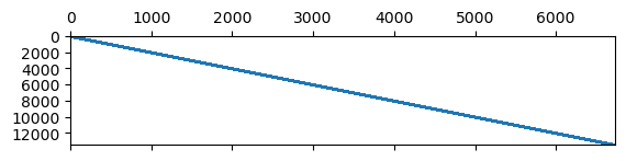
# getting a nice diagonal here requires sorting by the studend_id
plt.spy(A,aspect=0.1,markersize=0.2)
plt.show()
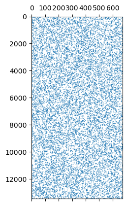
plt.spy(J,aspect=0.1,markersize=0.2)
plt.show()
<class 'scipy.sparse.csc.csc_matrix'>
(13464, 6732)
(13464, 673)
(13464,)
13464.0
13464.0
Estimating the model
Next we estimate our model using the OLS estiamtor formula. We first remove the last column of J (since the model we wrote does not pin down a constant we force the last course to have \psi=0). Solve the linear system using the formula
where M = [A,J] and \gamma = (\alpha,\psi).
So do the following:
- select the last column simply by doing
J = J[:,1:(nc-1]] - use
scipy.sparse.hstackto concatenate the matrices to create M - use
scipy.sparse.linalg.spsolveto solve a sparse linear system - extract \hat{\alpha} from \hat{\gamma} by selecting the first n_s terms
- merge \hat{\alpha} into
df_all - compute the variance of \hat{\alpha} in
df_all - compute the variance of the residuals
- What share of the total variation in grades can be attributed to difference in students?
df_all, M, gamma_hat = solution.question3(df_all,A,J,Y)
print(df_all['alpha_hat'].var(),df_all['resid'].var(),df_all['grade'].var())
df_all[["grade","class_id","student_id","major","firstname","alpha_hat"]]
1.347920639414136 0.2528814610764115 2.1867408049173007
| grade | class_id | student_id | major | firstname | alpha_hat | |
|---|---|---|---|---|---|---|
| 0 | -3.099938 | MQ2281 | 5 | SOCIAL SCIENCE OR HISTORY TEACHER EDUCATION | Francis | -3.626313 |
| 1 | -3.021075 | JP1499 | 5 | SOCIAL SCIENCE OR HISTORY TEACHER EDUCATION | Francis | -3.626313 |
| 2 | -0.042223 | HO0525 | 20 | ELEMENTARY EDUCATION | Cruz | -2.322520 |
| 3 | -1.842850 | BZ6573 | 20 | ELEMENTARY EDUCATION | Cruz | -2.322520 |
| 4 | 0.038426 | FM1995 | 21 | MISCELLANEOUS PSYCHOLOGY | Denise | -1.108136 |
| ... | ... | ... | ... | ... | ... | ... |
| 13459 | -2.082608 | JH2331 | 50684 | COMMUNICATIONS | Lavera | -2.349589 |
| 13460 | -1.478929 | IE5546 | 50687 | COGNITIVE SCIENCE AND BIOPSYCHOLOGY | Garold | -1.186850 |
| 13461 | -0.179943 | MG0664 | 50687 | COGNITIVE SCIENCE AND BIOPSYCHOLOGY | Garold | -1.186850 |
| 13462 | 5.874171 | CA0214 | 50693 | GENERAL BUSINESS | Gus | 3.840780 |
| 13463 | 4.786490 | JA7623 | 50693 | GENERAL BUSINESS | Gus | 3.840780 |
13464 rows × 6 columns
A simple evaluation of our estimator
To see what we are dealing with, we are simly going to re-simulate using our estimated parameters, then re-run our estimation and compare the new results to the previous one. This is in the spirit of a bootstrap exercise, onyl we will just do it once this time.
Please do:
- create Y_2 = M \hat{\gamma} + \hat{\sigma}_r E where E is a vector of draw from a standard normal.
- estimate \hat{\gamma}_2 from Y_2
- report the new variance term and compare them to the previously estimated
- comment on the results (not that because of the seed and ordering, your number doesn't have to match mine exactly)
df_all = solution.question4(df_all,M,gamma_hat)
df_all['alpha_hat2'].var(),df_all['resid2'].var()
(1.4806557269553007, 0.11529175149045187)
Noticed how even the variance of the residual has shrunk? Now is the time to remember STATS 101. We have all heard this thing about degree of freedom correction! Indeed we should correct our raw variance estimates to control for the fact that we have estimated a bunhc of dummies. Usually we use n/n-1 because we only estimate one mean. Here however we have estimated n_s +n_c - 1 means! Hence we should use
please do:
- compute this variance corrected for degree of freedom using your recomputed residuals
- compare this variance to the variance you estimated in quetion 3
- what does this suggest about your estimates in Q3?
solution.question4b(df_all)
Var2 with degree of freedom correction:0.256153158757004
Evaluate impact of academic measure on earnings
In this section we load a separate data set that contains for each student their earnings at age 35. We are intereted in the effect of \alpha on earnings.
Do the following:
- load the data the earnings data listed in the intro
- merge \alpha into the data
- regress earnings on \alpha.
df_earnings = solution.question5(df_all)
df_earnings
                            OLS Regression Results
==============================================================================
Dep. Variable:               earnings   R-squared:                       0.035
Model:                            OLS   Adj. R-squared:                  0.035
Method:                 Least Squares   F-statistic:                     245.3
Date:                Mon, 20 Sep 2021   Prob (F-statistic):           2.52e-54
Time:                        11:49:03   Log-Likelihood:                -9663.9
No. Observations:                6732   AIC:                         1.933e+04
Df Residuals:                    6730   BIC:                         1.935e+04
Df Model:                           1
Covariance Type:            nonrobust
==============================================================================
                 coef    std err          t      P>|t|      [0.025      0.975]
------------------------------------------------------------------------------
Intercept      0.1267      0.014      8.895      0.000       0.099       0.155
alpha_hat      0.1672      0.011     15.661      0.000       0.146       0.188
==============================================================================
Omnibus:                        0.805   Durbin-Watson:                   2.014
Prob(Omnibus):                  0.669   Jarque-Bera (JB):                0.843
Skew:                          -0.016   Prob(JB):                        0.656
Kurtosis:                       2.956   Cond. No.                         1.86
==============================================================================

Notes:
[1] Standard Errors assume that the covariance matrix of the errors is correctly specified.
| student_id | major | firstname | earnings | alpha_hat | |
|---|---|---|---|---|---|
| 0 | 5 | SOCIAL SCIENCE OR HISTORY TEACHER EDUCATION | Francis | -1.271396 | -3.626313 |
| 1 | 20 | ELEMENTARY EDUCATION | Cruz | 0.227663 | -2.322520 |
| 2 | 21 | MISCELLANEOUS PSYCHOLOGY | Denise | 0.011602 | -1.108136 |
| 3 | 28 | MATHEMATICS TEACHER EDUCATION | Kurtis | 0.998318 | 1.906966 |
| 4 | 30 | N/A (less than bachelor's degree) | Flor | 0.645380 | 0.850472 |
| ... | ... | ... | ... | ... | ... |
| 6727 | 50676 | ENGINEERING MECHANICS PHYSICS AND SCIENCE | Angelia | 1.501068 | 0.433212 |
| 6728 | 50681 | ELECTRICAL ENGINEERING TECHNOLOGY | Stacy | 0.954807 | -0.551522 |
| 6729 | 50684 | COMMUNICATIONS | Lavera | -1.701903 | -2.349589 |
| 6730 | 50687 | COGNITIVE SCIENCE AND BIOPSYCHOLOGY | Garold | 0.114382 | -1.186850 |
| 6731 | 50693 | GENERAL BUSINESS | Gus | 1.682317 | 3.840780 |
6732 rows × 5 columns
Bias correction - construct the Q matrix
We want to apply bias correction to refine our results. As we have seen in class thaqt we can directly compute the bias of the expression of interest.
under homoskedatic assumption of the error and hence we get the following expresison for the bias for any Q matrix:
When computing the variance of the measured ability of the student, we simply use a diagonal matrix on \gamma which selects only the ability part and removes the average.
do: 1. Construct such Q matrix. 2. check that \gamma Q \gamma' = \hat{Var}(\hat{a}).
# a small example if we had ns=5,nc=4
Qbis = solution.question6(ns=5,nc=4)
print(Qbis)

# the full Q
Q = solution.question6(ns,nc)

# comparing Q expression to df_all expression
1/(ns)*np.matmul( gamma_hat, np.matmul(Q,gamma_hat )), gamma_hat[range(ns)].var()
[[ 0.8 -0.2 -0.2 -0.2 -0.2  0.   0.   0. ]
 [-0.2  0.8 -0.2 -0.2 -0.2  0.   0.   0. ]
 [-0.2 -0.2  0.8 -0.2 -0.2  0.   0.   0. ]
 [-0.2 -0.2 -0.2  0.8 -0.2  0.   0.   0. ]
 [-0.2 -0.2 -0.2 -0.2  0.8  0.   0.   0. ]
 [ 0.   0.   0.   0.   0.   0.   0.   0. ]
 [ 0.   0.   0.   0.   0.   0.   0.   0. ]
 [ 0.   0.   0.   0.   0.   0.   0.   0. ]]


(1.34782052647301, 1.3478205264730092)
Bias correction - Variance share
We are now finally in the position to compute our bias. We have are matrix Q. Now we also need the variance of the residual! Given what we have learn in Question 4, we definitely want to use the formula with degree of freedom correction.
- Compute \sigma^2_r with the degree of freedom correction
- Invert M'M using
scipy.sparse.linalg - Compute B = \frac{\sigma^2}{N} \text{Tr}[ ( M'M )^{-1} Q] using
np.trace - Remove this from original estimate to get the share of variance explained by student differences!
Note that inversing a matrix is far longer than solving a linear system. You might need to be patient here!
B = solution.question7(M,Q,df_all)
B
/home/tlamadon/git/econ-21340/envs/lib/python3.8/site-packages/scipy/sparse/linalg/dsolve/linsolve.py:318: SparseEfficiencyWarning: splu requires CSC matrix format
  warn('splu requires CSC matrix format', SparseEfficiencyWarning)
/home/tlamadon/git/econ-21340/envs/lib/python3.8/site-packages/scipy/sparse/linalg/dsolve/linsolve.py:215: SparseEfficiencyWarning: spsolve is more efficient when sparse b is in the CSC matrix format
  warn('spsolve is more efficient when sparse b '


0.3119489890374221
gamma_hat[range(ns)].var() - B
1.0358715374355871
Bias correction - Regression coefficient
Finally, we look back at our regression of earnings on estimated academic ability. We have seen in class that when the regressor has measurment error this will suffer from attenuation bias. Here we now know exactly how much of the variance is noise thanks to our bias correction.
The attenuation bias is given by :
We then decide to compute a correction for our regression using our estimated B. This means computing a corrected parameters as follows:
Do:
- compute the corrected \hat{\beta}^{BC}
- FIY, the true \beta I used to simulate the data was 0.2, is your final parameter far? Is is economically different from the \hat{\beta}^{Q5} we got in Question 5?
Conclusion
I hope you have learned about the pitfalls of over-fitting in this assignment! There are many and they can drastically affect the results and the conclusion of an empirical analysis.
This is the end of the class, I hope you enjoyed it and that you learned a thing or twom, have a nice summer!