Preliminary notes on synthetic control

import pandas as pd
import matplotlib.pyplot as plt
import numpy as np

data = pd.read_csv('../data/cigs.csv')
data

	state	year	cigs	loggdppercap	retprice	pctage1524	beerpercap	cigsalespercap88	cigsalespercap80	cigsalespercap75
0	AL	1970	89.8	9.679	89.344	0.175	18.96	112.1	123.2	111.7
1	AL	1971	95.4	9.679	89.344	0.175	18.96	112.1	123.2	111.7
2	AL	1972	101.1	9.679	89.344	0.175	18.96	112.1	123.2	111.7
3	AL	1973	102.9	9.679	89.344	0.175	18.96	112.1	123.2	111.7
4	AL	1974	108.2	9.679	89.344	0.175	18.96	112.1	123.2	111.7
...	...	...	...	...	...	...	...	...	...	...
1204	WY	1996	110.3	9.914	81.000	0.174	24.98	114.3	158.1	160.7
1205	WY	1997	108.8	9.914	81.000	0.174	24.98	114.3	158.1	160.7
1206	WY	1998	102.9	9.914	81.000	0.174	24.98	114.3	158.1	160.7
1207	WY	1999	104.8	9.914	81.000	0.174	24.98	114.3	158.1	160.7
1208	WY	2000	90.5	9.914	81.000	0.174	24.98	114.3	158.1	160.7

1209 rows × 10 columns

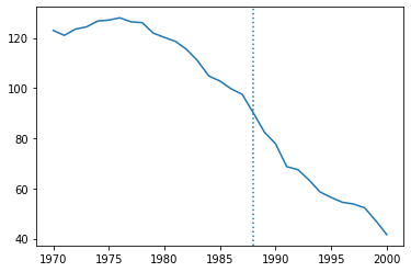
dcal = data.query("state=='CA'")
plt.plot(dcal['year'],dcal['cigs']) 
plt.axvline(1988,linestyle=":")
plt.show()

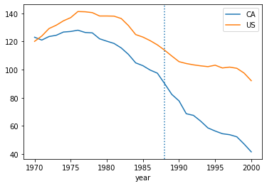
dcal = data.query("state=='CA'")
plt.plot(dcal['year'],dcal['cigs'],label="CA") 
data.query("state != 'CA'").groupby('year')['cigs'].mean().plot(label="US")
plt.axvline(1988,linestyle=":") 
plt.legend()
plt.show()

Checking pretrends

We can regress using the other states as control.

data['D'] = (data['state']=='CA') & (data['year']>=1988)
data['T'] = (data['state']=='CA') 

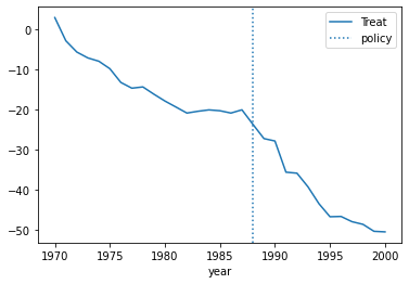
To evaluate the pre-trend, we can estimate the coffecient of the interaction with the values leading to the event.

import statsmodels.formula.api as smf

# Initialise and fit linear regression model using `statsmodels`
model = smf.ols("cigs ~ C(year)  + C(year):C(T)", data=data)
model = model.fit()

data_cal = data.query("state == 'CA'").copy()
data_cal['dep'] = model.predict(data_cal) - model.predict( data_cal.eval("T=False") )

data_cal.plot(x='year',y='dep',label="Treat")
plt.axvline(x=1988, linestyle=':',label="policy")
plt.legend()

<matplotlib.legend.Legend at 0x7f60f1d68d90>

Construct non treated outcome using observables

In this section we think about directly constructing a control group as a weighted sum of available non treated units. A simple choice would be to pick the state with the most similar observables. Or we could weight becased on the distance on obserbales.

Let's try both of these approaches.

Next we might want to change the way we construct our non-treated counterfactual for California. First we could choose to use observables characteristics to be added to our framework.

loggdppercap retprice pctage1524 beerpercap

# we start by computing pair-wise distances between observations